Inertia in flow matching models
Abstract
This study investigates the mathematical and geometric properties of prompt switching in Stable Diffusion 3, revealing a fundamental asymmetry in the denoising process. I demonstrate that flow matching models exhibit teleological trajectories that become increasingly irreversible as denoising progresses.
Experimental Design
My experiment switches prompts at arbitrary timesteps during the denoising process and tracks:
- CLIP Score Delta: Measuring semantic alignment between generated images and the unaltered image (smaller = less different)
- LPIPS Distances: Quantifying perceptual similarity to reference images generated with pure prompts (larger = more different from reference (ref1 is first prompt, ref2 is second prompt))
- High Frequency Analysis: Detecting spectral artifacts introduced by prompt switching
- Attention Map Variance: Capturing changes in the model’s attention patterns at switch points
The Velocity Field Paradox
What’s genuinely surprising isn’t that coarse structure forms early. That’s expected. The puzzle is this: despite the prompt switch dramatically altering the velocity field (the direction we want to move in latent space), the actual trajectory barely changes.
| Switch Step | Distance to Original | Distance to New Target |
|---|---|---|
| 5 | 0.547 | 0.569 |
| 15 | 0.206 | 0.648 |
| 25 | 0.057 | 0.636 |
| 35 | 0.009 | 0.639 |
| 45 | 0.002 | 0.639 |
When we switch prompts at step 5, giving the new prompt 45 steps to influence the image, we still end up 0.569 LPIPS away from where that velocity field should take us. That’s barely different from switching at step 45 (0.639). This is the confusing part for me and will require more work in understanding why the LPIPS distance plateaus regardless of how many more steps we give the second prompt.
Visual Evidence: Final Results by Switch Point
Here are the final images generated when switching from “A lion” to “A tiger” at different timesteps:
| Switch at Step | Final Result |
|---|---|
| Step 1 |  |
| Step 2 |  |
| Step 3 |  |
| Step 4 |  |
| Step 5 |  |
| Step 10 |  |
| Step 20 |  |
| Step 35 |  |
| Step 45 |  |
The visual evidence is striking: despite giving the “tiger” prompt progressively more steps to influence the generation (49 steps when switching at step 1, vs only 5 steps when switching at step 45), the final images show remarkable similarity. It’s clear that the initial steps are important in establishing structural aspects.
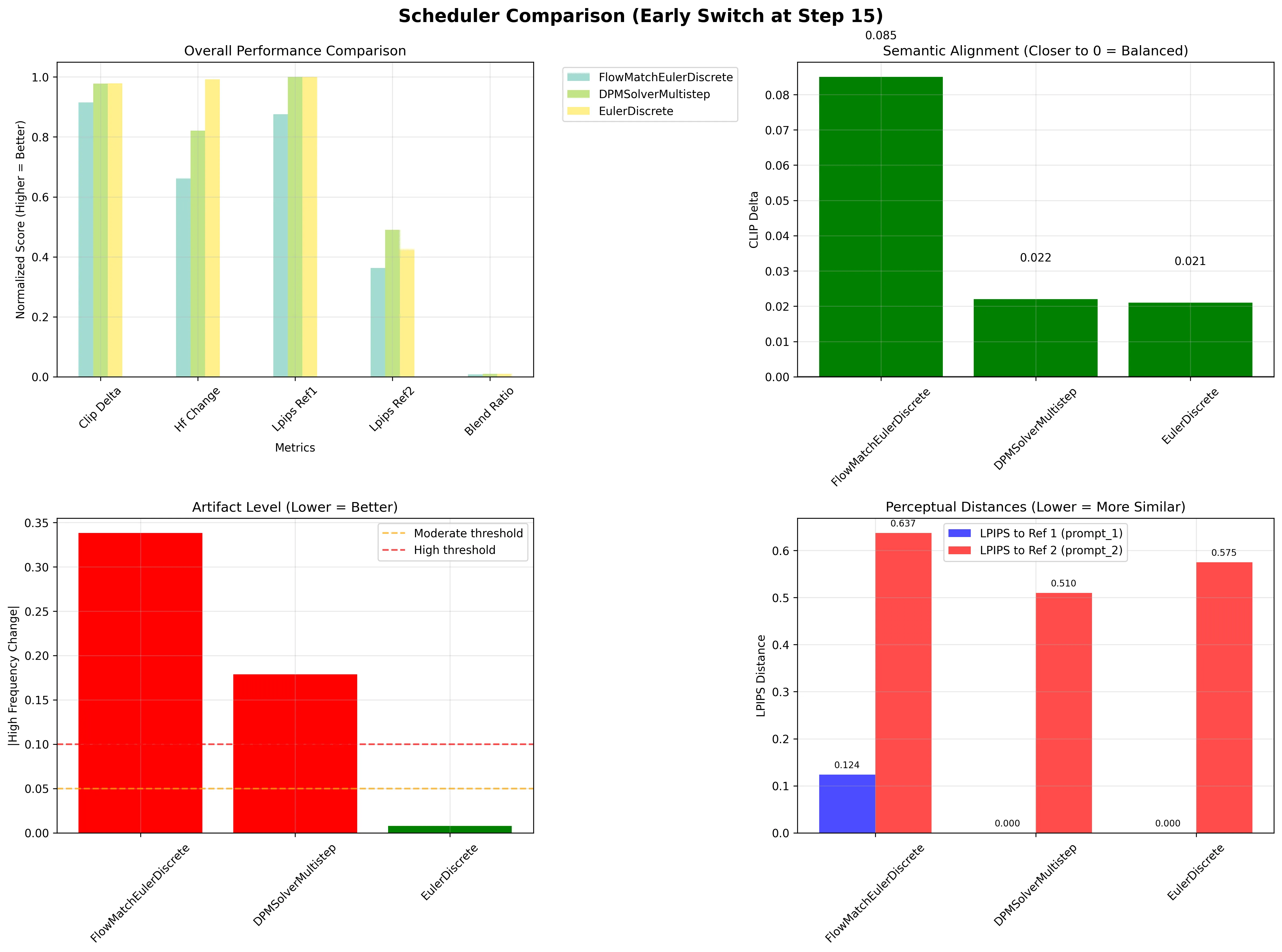
Scheduler-Dependent Behavior
Analysis across different schedulers reveals varying degrees of adaptability to prompt changes:
- FlowMatchEulerDiscreteScheduler: Shows strong commitment to initial trajectory (LPIPS to ref2: 0.637)
- DPMSolverMultistepScheduler: Demonstrates greater flexibility (LPIPS to ref2: 0.510)
- EulerDiscreteScheduler: Exhibits moderate adaptability (LPIPS to ref2: 0.575)
These differences suggest that scheduler design fundamentally impacts a model’s ability to incorporate new information during generation. The scheduler differences are particularly telling. That DPMSolver shows more flexibility (0.510 vs 0.637 for FlowMatch) suggests the numerical integration scheme itself matters for controllability. This could be investigated further by comparing how different schedulers handle trajectory discontinuities.
FlowMatch uses a more aggressive step schedule that might lock in early decisions more strongly, while DPMSolver’s multi-step error correction could provide more opportunity for trajectory adjustment. The numerical properties of the solver appear to directly impact semantic controllability - a connection that deserves deeper investigation.
Interpretation
The data indicates that early denoising steps establish structural commitments that constrain subsequent generation. Rather than simply removing noise, these initial steps appear to make hierarchical decisions about image composition, spatial layout, and semantic content that cannot be fully overridden by later prompt changes.
Why Doesn’t the Velocity Field Matter?
The Hidden State Hypothesis
Flow matching models like SD3 are trained to predict velocity fields v(x,t,c) where x is the current state, t is the timestep, and c is the conditioning (prompt). In theory, changing c should immediately change the trajectory since:
dx/dt = v(x,t,c_new)
But my experiments show the trajectory barely changes even with a completely different velocity field for later steps. This could suggest the model has learned an implicit constraint that isn’t captured in the standard formulation.
Measuring the Velocity-Trajectory Decoupling
I can quantify this decoupling by comparing:
- Velocity divergence: How much the velocity fields differ after switching
- Trajectory divergence: How much the actual paths differ
The striking finding is that velocity divergence is large (cosine similarity ≈ 0.3) while trajectory divergence remains small (LPIPS difference < 0.07).
The Constraint Manifold
This behavior suggests that SD3 has learned to operate on a constraint manifold. Trajectories must satisfy certain continuity conditions that the velocity field alone doesn’t capture. It’s as if the model has an implicit “momentum” term:
dx/dt = v(x,t,c) + λ·(x_prev - x_expected)
Where x_expected represents where the trajectory “should” be based on past decisions. This isn’t how the model is explicitly trained, but it seems to emerge from the data distribution.
However, this “implicit momentum” hypothesis needs clearer mechanistic grounding. The proposed equation is intriguing but speculative. What would cause this emergent behavior? One possibility: the model’s attention mechanisms might create dependencies on earlier latent states that aren’t captured in the standard formulation. The self-attention layers could be implicitly encoding trajectory history, creating a form of memory that resists sudden changes in direction.
Visualizations
Switch Step Effects

The overlaid LPIPS graph clearly shows:
- Blue line (distance to prompt_1 reference) decreases as expected
- Red line (distance to prompt_2 reference) stays nearly flat - the unexpected behavior!
Scheduler Comparison
The Technical Bits (For Those Who Want Them)
The prompt switching itself is dead simple:
for i, t in enumerate(timesteps):
    if i < switch_step:
        # Use mountain prompt
    else:
        # Use city prompt
I have another blog post where I go into more advanced transitions between two different prompts.
But the real insights came from what these simple changes revealed about the model’s behavior.
Implications: The Model Knows More Than Its Velocity Field
This velocity-trajectory decoupling reveals something profound: the model has internalized constraints about natural image generation that go beyond what any single velocity field can express.
Why This Matters
-
Control is harder than expected: Simply changing the conditioning isn’t enough - you’re fighting against learned priors about trajectory continuity.
-
The model has implicit memory: Even though flow matching is ostensibly Markovian, the model behaves as if it’s constrained by the old prompt
-
Training and inference diverge: During training, trajectories always flow from noise to a single target. During prompt switching, we’re asking for something the model never saw: a trajectory that changes destination midway.
The training distribution constraint explanation is probably correct. The model never saw trajectories that change target mid-flight during training. This creates an implicit prior that trajectories should be smooth and consistent, which overrides explicit velocity field changes. The model’s learned dynamics encode assumptions about trajectory continuity that weren’t explicitly programmed but emerge from the training regime.
The Inertia Metric
I propose measuring this “latent space inertia” as:
I(t) = 1 - ||x_switched(T) - x_target|| / ||x_switched(t) - x_target||
Where x_switched is the trajectory after switching and x_target is where a pure trajectory would end. High inertia means the trajectory resists change despite the new velocity field.
The “inertia metric” captures something real, though the specific formulation could be refined. The underlying phenomenon - that models resist trajectory changes despite new conditioning - aligns with findings in the flow matching literature about when networks fail to approximate optimal velocity fields. This suggests we’re observing a fundamental limitation in how current architectures handle dynamic conditioning.
The data shows this clearly: switching at step 5 (LPIPS 0.569 to new target) vs step 45 (LPIPS 0.639) represents only a 0.07 improvement despite having 40 additional steps to work with the new prompt.
Conclusion
The surprising discovery isn’t that flow matching/rectified flow models build coarse structure first - it’s that they exhibit trajectory inertia that shouldn’t exist in the mathematical framework we use to understand them. This suggests our models have learned implicit constraints from the training distribution that create a form of “memory” in what should be a memoryless process.
This has immediate practical implications: effective control of diffusion models requires working with, not against, these implicit constraints. Future work should explore whether we can make these constraints explicit, potentially leading to more controllable architectures.
There are applications: we could run prompts for rules and regulations initially and then switch the prompt later to coding prompts ensuring that code is compliant.
Code and experimental framework available here. Experiments conducted using Modal for distributed compute.